Simple Linear Regression

This is the most basic model out there as it has only two variables and even a normal human being can carry out the math included in this model easily. This model just tries to create a straight line with the equation Y=mX + c where Y is the target variable, X is the feature, m is the slope and c is just a constant.

In this image above, the model tries to draw a line with feature height and target weight to predict future results. The constant c over here is 80 and the slope m is 2. With this data, the model is sure that it can predict weight for any value of height if the linear relation is followed thoroughly. 

You might have noticed that not all the points are on the line so how does the model decides what line to pass as result. What the linear regression model does it tries lots and lots of results and select the best of them. Obviously the best line is the one that has the least error and the error is the sum of the square of the difference between the actual value and the real value. 

As you can see, y(i) is the real value and hat(y(i)) is the value that the model suggests. The green dotted line is the error. To get the best line, the least square error is selected considering all the green dotted lines. So basically, from a number of lines, the best line is selected and that line might change on adding new data to training dataset.

As we all know that this is the most basic model so it sure comes with some drawbacks. The major drawback is that it is not really made for more than one feature training which is never the case in real world data. But it still is the base for multiple linear regression model which overcomes this limitation. Another drawback is it not compatible with outliers in data. 

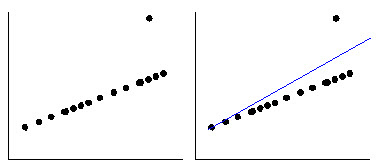
Outliers in the data are nothing but irregularities which disrupt the model results and are needed to be removed before training the model.

This is what an outlier does to a result. You can determine the result should be passing from the line very close to all the points but due to a single outlier, the accuracy is degraded.

Now that you know how the model works let's get to implementing it. I will be using a simple dataset of years of experience and salary which you can get from below.

The next step after getting the dataset is preprocessing it. We will not need to worry about missing or categorical values as there are none. Nor we need to scale the data as there is only one feature. so we will just get the dataset and split it in training and test data.

# Importing the libraries
import numpy as np
import matplotlib.pyplot as plt
import pandas as pd

# Importing the dataset
dataset = pd.read_csv('Salary_Data.csv')
X = dataset.iloc[:, :-1].values
y = dataset.iloc[:, 1].values

# Splitting the dataset into the Training set and Test set
from sklearn.cross_validation import train_test_split
X_train, X_test, y_train, y_test = train_test_split(X, y, test_size = 1/3, random_state = 0)

# Fitting Simple Linear Regression to the Training set
from sklearn.linear_model import LinearRegression
regressor = LinearRegression()
regressor.fit(X_train, y_train)

# Predicting the Test set results
y_pred = regressor.predict(X_test)

# Visualising the Training set results
plt.scatter(X_train, y_train, color = 'red')
plt.plot(X_train, regressor.predict(X_train), color = 'blue')
plt.title('Salary vs Experience (Training set)')
plt.xlabel('Years of Experience')
plt.ylabel('Salary')
plt.show()

# Visualising the Test set results
plt.scatter(X_test, y_test, color = 'red')
plt.plot(X_train, regressor.predict(X_train), color = 'blue')
plt.title('Salary vs Experience (Test set)')
plt.xlabel('Years of Experience')
plt.ylabel('Salary')
plt.show()

I have posted individual post for every step in the data preprocessing section. The iloc is used to select part of the dataset and using [ : , : -1] means to get all rows (the first colon) and get all columns except the last (second colon with the -1). Using random_state=0 in the train_test_split will make sure that the data is splitted as it is and mine and your results will be the same. 

The LinearRegression is available in sklearn.linear_model library and has a function fit which is used to train the model on the data specified in the argument. Predict is another function that is used to predict the target value based on the trained model for the features specified in the argument. The results are stored in the y_pred variable and we can actually visualize the results in the form of a graph.

Scatter plot is a graph where there will be points for each and every entry and plot function is used to dwar a line on the graph. On plotting the training graph you will see a figure like this.

With just four lines,you can train a model and predict results based on it. But using a model without the knowledge of what's going on is not recommended. So one should get the basics clear enough to understand where and how to use it.

Hope you like this post and do tell if you find it useful. Everybody stay Awesome!